computing the relative dem and orthophoto#
Once you have the relative orientation, you can use Malt to compute a relative DEM and orthoimages:
mm3d Malt Ortho "OIS.*tif" Relative DirMEC=MEC-Relative NbVI=2 ZoomF=4 DefCor=0 CostTrans=4 EZA=1 SzW=3 Regul=0.1
This will run Malt on all of the images, using the orientation described in Ori-Relative. The DEM and
correlation models will be output to MEC-Relative, and the orthophotos will be output to Ortho-MEC-Relative.
The other parameters used here are:
NbVI (number of visible images):
Maltdefaults to only running where 3 or more images are visible (NbVI=3), but it is usually fine to go with 2 images.ZoomF (final zoom level): At this stage, we don’t necessarily need the DEM to be processed to full resolution - a lower-resolution version (
ZoomF=4orZoomF=8) will suffice.DefCor (default correlation value): the default correlation value to use in pixels that are uncorrelated.
CostTrans (transition cost): the cost to transition from correlation to decorrelation. Higher values means that more areas are included (because it is ‘harder’ to transition to decorrelation), though it may also increase the noise in the final result.
EZA (export Z absolute):
EZA=1argument ensures that the values in the DEM are absolute (in the units of the coordinate system), rather than scaled.SzW (correlation window size): the half-size of the window of the correlation window.
SzW=3means using a 7x7 correlation window; larger window sizes increase the likelihood of finding matches in areas with poor contrast (i.e., over glaciers), but also tend to smooth out the elevation.Regul (regularization factor): the regularization factor (penalty) to use for the transition term. Higher values tend to smooth out the terrain.
Alternatively, using spymicmac.micmac.malt():
from spymicmac import micmac
micmac.malt('OIS.*tif', 'Relative',
    zoomf=4,
    dirmec='MEC-Relative',
    cost_trans=4,
    szw=3,
    regul=0.1
)
Once this command finishes, you will have two new directories: MEC-Relative and Ortho-MEC-Relative. The DEM
and associated correlation masks are found in MEC-Relative, while the orthophotos are found in
Ortho-MEC-Relative.
You can visualize the DEM in a GIS software (for example, QGIS):
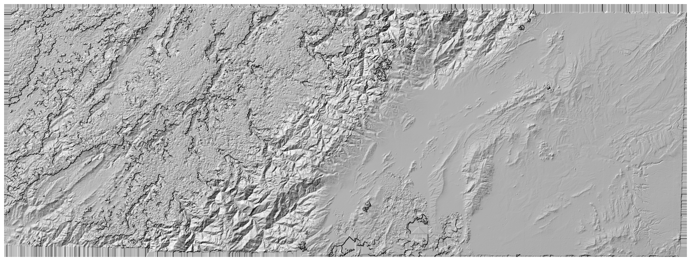
Assuming that the relative orientation, visualized with AperiCloud, is in good shape, the DEM hillshade should
look similar to a real-world hillshade of the study area - this is how spymicmac.register.register_relative()
works to register the images to real-world control points and compute the absolute orientation.
creating the orthomosaic using Tawny#
You can also create a relative orthomosaic using the images in Ortho-MEC-Relative. After calling Malt, these
images will only be the individual images orthorectified using the extracted
DEM.
To generate an orthomosaic, we use Tawny:
mm3d Tawny Ortho-MEC-Relative Out=Orthophotomosaic.tif RadiomEgal=0
Here, we use RadiomEgal=0 to use the images as-is, rather than attempting to balance the radiometry (as this
can lead to undesirable results).
Alternatively, using spymicmac.micmac.tawny():
from spymicmac import micmac
micmac.tawny('MEC-Relative')
Finally, you might need to re-combine the image tiles using
spymicmac.micmac.mosaic_micmac_tiles() (or mosaic_micmac_tiles) depending on
how large they are:
mosaic_micmac_tiles Orthophotomosaic -imgdir Ortho-MEC-Relative
As with the DEM, you can visualize the orthomosaic in a GIS software:
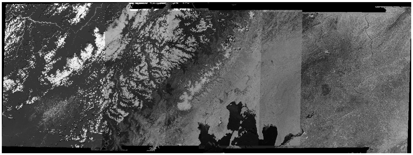
Once this is complete, you can move on to the next step: registering the DEM or orthoimage and automatically
finding control points using an external DEM and satellite image.