automatically finding control points

At this point, you should have successfully run mm3d Malt and mm3d Tawny to generate a relative orthophoto and DEM. You should also have run spymicmac.micmac.mosaic_micmac_tiles() (or mosaic_micmac_tiles) if needed - otherwise, spymicmac.register.register_relative() (or register_relative) will most likely fail.

In order to run spymicmac.register.register_relative(), you will need a number of files, detailed in the section below. After that, this document will describe the process that spymicmac.register.register_relative() uses to find GCPs and iteratively refine the orientation.

necessary files

reference orthoimage and DEM

At the risk of stating the obvious, the reference DEM (or orthoimage, if using one) should cover your study area.

The reference orthoimage can be a high-resolution orthomosaic, or it can be a comparatively low-resolution satellite image. spymicmac.register.register_relative() has been tested on both Landsat-8 and Sentinel-2 images, with satisfactory results for both.

In general, the results will depend in part on the accuracy of the control points - so if your reference orthoimage is highly accurate and of a similar resolution to your air photos, the more accurate the result will be.

Similar rules apply for the reference DEM - the more accurate the DEM, the better the final result.

spymicmac.data has methods available for accessing high-quality, publicly available DEMs from the following sources:

Copernicus Global 30m DSM

spymicmac.data.download_cop30_vrt(), will download and create a VRT of the Copernicus Global 30m DSM tiles that intersect the footprints of the images:

from spymicmac import data
data.download_cop30_vrt()

With no arguments, this will use the images in the current folder, download the footprints from the corresponding USGS dataset, and intersect this with the Copernicus DSM tiles. If you are using a non-USGS dataset, or you have already downloaded the footprints for your images, or you have a rough study area outline, you can pass this using the footprints argument.

Because the vertical datum for the Copernicus DSM is height above the EGM2008 Geoid, you will need to convert the VRT to height above the WGS84 ellipsoid, using spymicmac.data.to_wgs84_ellipsoid():

from spymicmac import data
data.to_wgs84_ellipsoid('Copernicus_DSM.tif')

This will create a file Copernicus_DSM_ell.tif, which represents the elevations referenced to the WGS84 ellipsoid.

Note

Before converting the vertical datum, it is recommended to first re-project the DSM to a local coordinate reference system, using for example gdalwarp:

gdalwarp -t_srs EPSG:32629 -tr 30 30 -r bilinear Copernicus_DSM.vrt Copernicus_DSM.tif

Polar Geospatial Center DEMs

If you are working in polar regions, you can use spymicmac.data.download_pgc_mosaic() to download and create a VRT of mosaic tiles from the Polar Geospatial Center using one of two flavors:

• adem: the ArcticDEM, covering most areas north of 60°N.

• rema: the Reference Elevation Model of Antarctica (REMA), covering Antarctica and some sub-Antarctic islands.

Both the ArcticDEM and REMA mosaics are available at resolutions of 2, 10, or 32m. The default (res=2) is 2m, but because of the size of the files you may wish to specify a lower resolution:

from spymicmac import data
data.download_pgc_mosaic('adem')

As with the Copernicus DSM, with no arguments this will use the images in the current folder, download the footprints from the corresponding USGS dataset, and intersect this with the corresponding tile boundaries.

If you are using a non-USGS dataset, or you have already downloaded the footprints for your images, or you have a rough study area outline, you can pass this using the footprints argument.

Both the ArcticDEM and REMA are given as height above the WGS84 ellipsoid, so no conversion is required here.

image footprints

This should be a vector dataset (e.g., shapefile, geopackage - anything that can be read by geopandas.read_file). The footprints do not have to be highly accurate - most of the routines in spymicmac.register() have been developed using USGS datasets/metadata, which are only approximate footprints.

The main use for the footprints in spymicmac.register.register_relative() is in the call to spymicmac.orientation.transform_centers(), which uses RANSAC to estimate an affine transformation between the footprint centroids and the relative camera centers estimated by mm3d Tapas.

As long as the distribution of the footprints/centroids is approximately correct, this step should work according to plan.

Note

Some USGS Aerial Photo Single Frames (as well as the KH-9 Hexagon images) have footprints that are incorrectly placed, or the images have been scanned but not georeferenced. In this case, you may need to create your own footprints. It is most likely worth checking the metadata for these images before you start working.

exclusion and inclusion masks (optional)

Finally, in areas with lots of water or terrain that has changed substantially (e.g., glaciers), spymicmac.register.register_relative() can use both exclusion and inclusion masks to avoid searching for matches on unstable terrain. Just like with the footprints, these files should be any data format that can be read by geopandas.read_file.

The exclusion mask should be polygons of glaciers, landslides, or other terrain that should be excluded from the search. Areas covered by this mask will be excluded from the search.

The inclusion mask should be polygons of land - any terrain that should be included in the search. Areas that are not covered by this mask will be excluded from the search.

relative to absolute transformation

The first step in spymicmac.register.register_relative() to use spymicmac.orientation.transform_centers() to transform between the relative and absolute spaces, using the centroids of the footprint polygons and the camera positions estimated by mm3d Tapas.

The initial transformation is plotted for review:

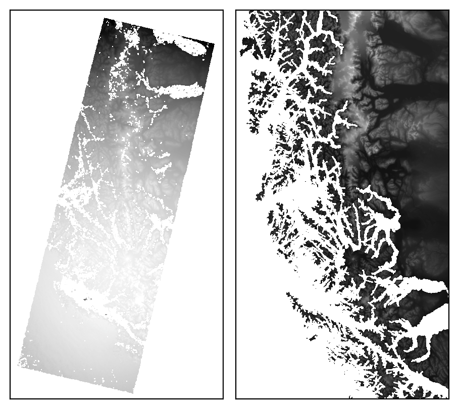
and the relative image, re-projected to the extent and CRS of the reference image, is also saved for checking.

Because the footprints are most likely approximate, especially for historic datasets, this step uses RANSAC with a fairly large residual threshold. The goal is to create a rough transformation of the relative orthophoto that can be used for the gridded template matching step.

template matching

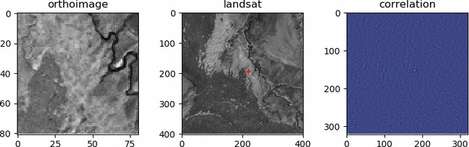
Once the relative orthophoto has been roughly transformed to absolute space, spymicmac.register.register_relative() finds matches between the orthophoto and the reference image using spymicmac.matching.find_matches(). The size of each template is 121x121 pixels, while the size of the search window is set by dstwin.

Each template and search image are first run through spymicmac.image.highpass_filter(), to help minimize radiometric differences between the two images (and maximizing the high-frequency variation). After that, the template and search image are passed to OpenCV matchTemplate, and the best match is found using normalized cross-correlation.

The correlation value of each potential match is then compared to the standard deviation of all of the correlation values from the search image. This value (z_corr) is then used to filter out poor matches later on, as higher quality matches are more likely to represent larger departures from the background correlation value:

iterative outlier removal

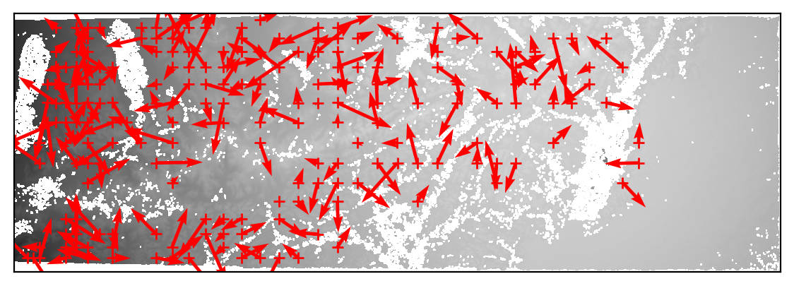
After the potential matches are found, a number of filtering steps are used to refine the results. First, any matches where the DEM does not have a value are removed. Then, an affine transformation between the relative orthoimage and reference orthoimage locations is estimated using RANSAC, to help remove obvious blunders.

Next, mm3d GCPBascule is called, which transforms the camera locations to the absolute space. The residuals for each GCP are then calculated, and outliers more than 3 normalized median absolute deviations (NMAD) from the median residual value are discarded, and mm3d GCPBascule is called again.

This is followed by a call to mm3d Campari using spymicmac.micmac.campari(), and again residuals more than 3 NMAD from the median residual value are discarded.

After this, this process (mm3d GCPBascule -> mm3d Campari -> outlier removal) is run up to 5 more times, until there are no further outliers found.

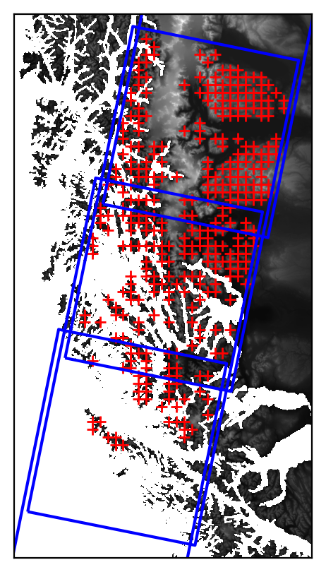
final result

Once the outliers have been removed, the final GCP locations are stored in a number of files:

• auto_gcps/AutoGCPs.xml

• auto_gcps/AutoGCPs.txt

• auto_gcps/AutoGCPs.shp (+ other files)

• AutoMeasures.xml – the GCP locations in each of the individual images

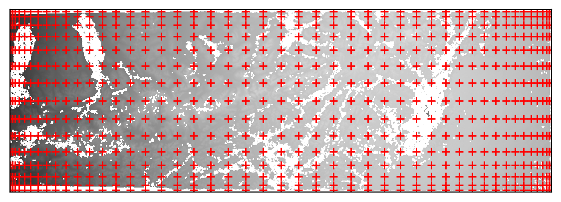
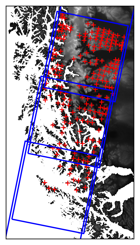
The final location of the GCPs is shown in both the relative image space:

as well as the absolute space:

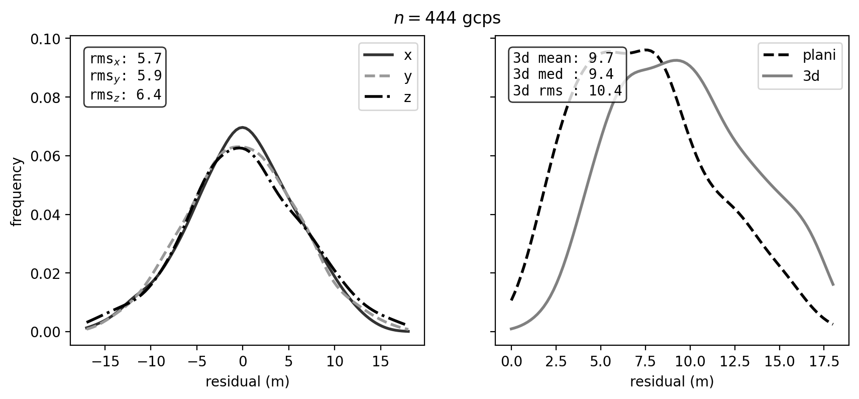
And, the distribution of residuals is plotted for each of the x, y, and z dimensions, as well as the planimetric and three-dimensional residuals:

If there are still problematic GCPs, you can manually delete them from AutoMeasures.xml and re-run mm3d GCPBascule and mm3d Campari.

The next step will be to run mm3d Malt using the Ori-TerrainFirstPass directory, to produce the absolute orthophoto and DEM.

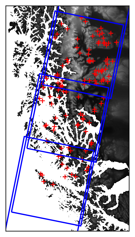
using check points

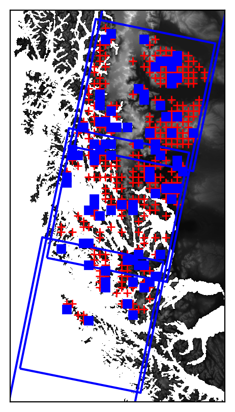
To evaluate the results of the registration and bundle block adjustment, you can also use check points (use_cps=True). This will randomly select a proprotion of the initial match points (cp_frac=0.2), and evaluate the residuals of these check points after the iterative bundle block adjustment is finished.

Check points are plotted as blue squares in the GCP location plots:

As with the GCPs, the distribution of residuals is also plotted:

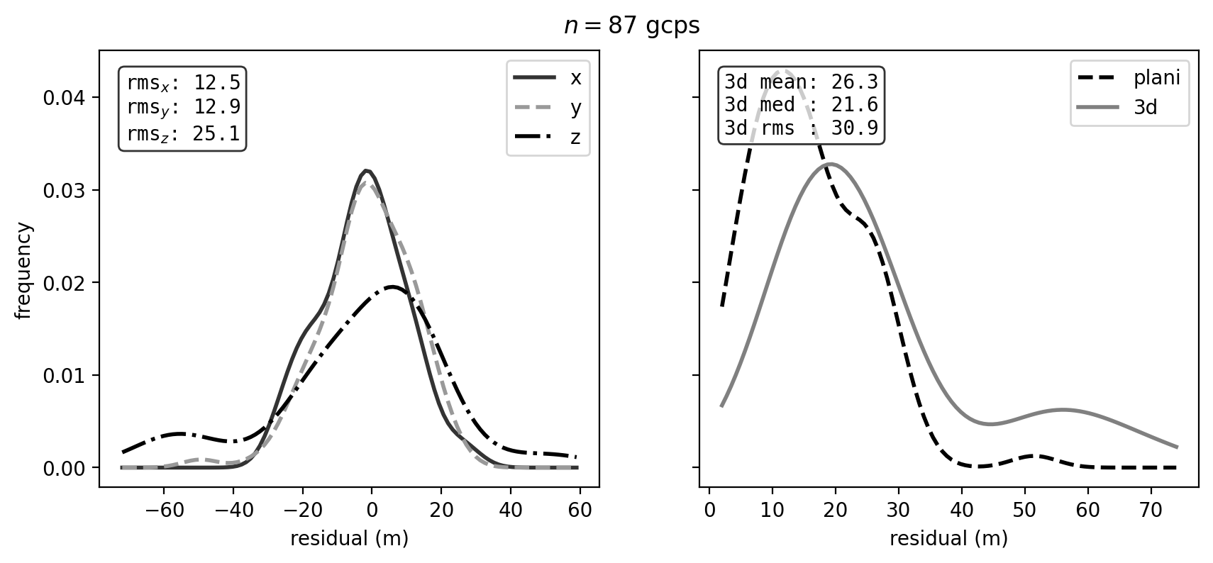
Note that because the check points are randomly selected from the initial matches, it is possible that there will be large residuals due to spurious matches or other issues with the points.

search strategies

Five different strategies for template matching are available:

• regular grid (strategy='grid') - a regular grid of points, spaced by density pixels (default value: 200), is used to register the relative image to the reference image. This is the default option.

• random points (strategy='random') - potential points are generated randomly throughout the image. In this case, density is the approximate total number of points desired, rather than the spacing.

• Chebyshev nodes (strategy='chebyshev'). A grid is generated by using the formula for the \(n\) Chebyshev nodes of the second kind, where \(n\) is calculated for each image dimension by dividing the dimension by density and taking the integer value. This has the benefit of increasing the density of search points at the border of the image domain and decreasing the density in the center, which can help to lessen the effects of doming in the bundle block adjustment.

• manually identified points (fn_gcps) - template matching is performed using the point locations passed through either a CSV or shapefile/geopackage.

• orb (use_orb=True) - potential points are identified within a grid (spaced by density pixels) using skimage.feature.ORB. This has the benefit of selecting clear/obvious features, though it may also be more time intensive owing to the higher number of potential matches generated.

The plots below illustrate the difference in distributions between the regular grid (left), random points (center), and chebyshev (right) strategies, run using the same initial parameters:

With strategy='chebyshev', the GCPs are more dense along the edges of the image overlap, and less densely spaced towards the middle of the overlapping area: