KH-9 mapping camera pre-processing steps

There are a number of necessary pre-processing steps when working with KH-9 mapping camera imagery. Distortions in the film, caused by storage and other conditions, must be corrected to be able to accurately process the images. After resampling, it is also possible to remove the Reseau marks from the images, in order to improve the final results.

Finally, because of the size of the film (approx. 9”x18”), the images are scanned in two halves that must be joined together. And finally, it can also be helpful to improve contrast in the images, in order to help improve the final results.

If you have a number of images, the convenience tool preprocess_kh9 will do the following steps, starting from tarballs of the image halves (as downloaded from USGS):

• extract the images from tar files (moving the tar files to a new folder, “tarballs”)

• join the scanned image halves

• detect the location of Reseau markers in each image

• erase the detected Reseau markers from each image

• filter images using a 1-sigma Gaussian Filter to reduce noise in the scanned images

• resample the images to a common size, using the Reseau marker locations

• call mm3d Tapioca to find tie points in the images

• call mm3d Tapas, to calibrate the camera model and find the relative image orientation

• call mm3d AperiCloud to create a point cloud using the calibrated camera model and relative camera positions

Some of these steps, including the relevant spymicmac functions, are detailed below.

image joining

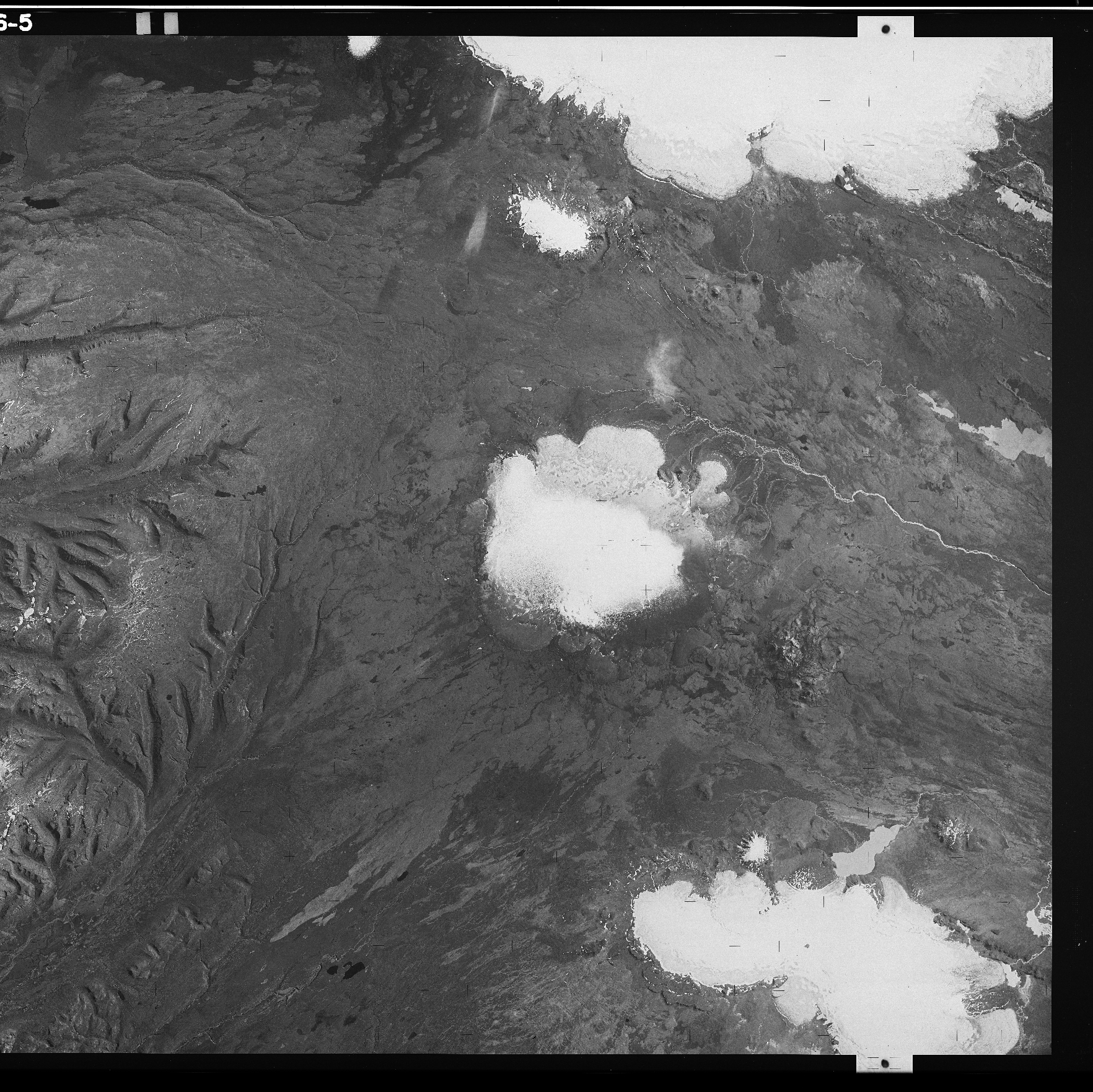
Because of the large size of the film, USGS scans the images in two halves with a small amount of overlap, as shown in the example below.

In spymicmac, the function to join the images is spymicmac.image.join_hexagon(), with a corresponding command-line tool join_hexagon.

Normally, the scans are labelled ‘a’ and ‘b’, with ‘a’ corresponding to the left-hand scan, and ‘b’ corresponding to the right-hand scan. This is what spymicmac.image.join_hexagon() is expecting - that the overlap between the two halves is the right-hand side of image ‘a’, and the left-hand side of image ‘b’.

After calling join_hexagon, the image should look something like this:

As there is sometimes a difference in brightness between the two halves, spymicmac.image.join_hexagon() has the option to blend the two halves over the overlap by averaging the values from the two halves, starting from 100% of the value of image ‘a’, linearly increasing to 100% of the value of image ‘b’ at the end of the overlapping part.

reseau field

To help correct some of the distortion in the images caused by film storage, spymicmac.matching() includes a routine to automatically find the Reseau markers in the image and use their locations to resample the images using spymicmac.resample.resample_hex().

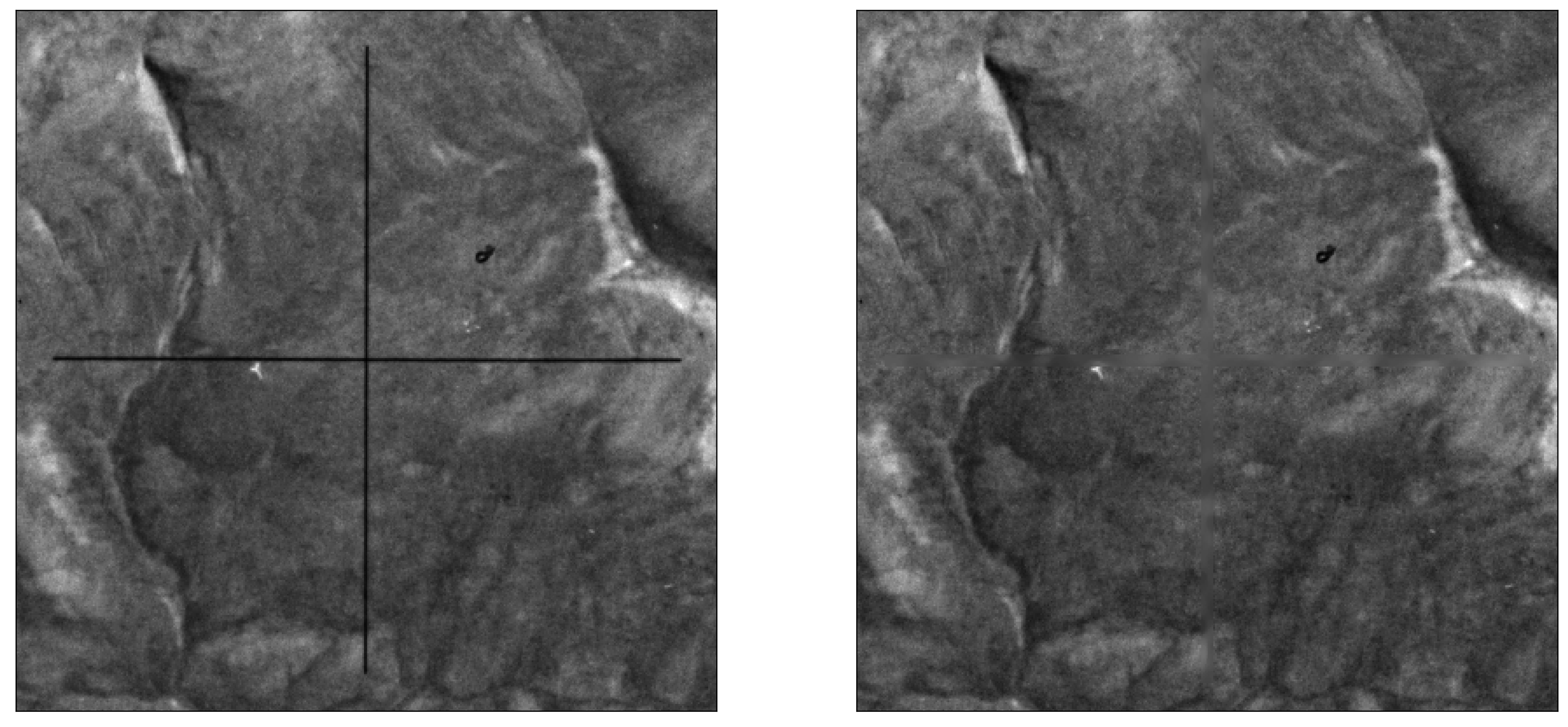
In the images below, you can see the difference between the expected location of each Reseau marker and the automatically detected locations:

To run the routine, use either spymicmac.matching.find_reseau_grid() or find_reseau_grid. This will produce a MeasuresIm file that will be read by spymicmac.resample.resample_hex().

Note

Before running spymicmac.resample.resample_hex(), you will also need to run generate_micmac_measures in order to generate the MeasuresCamera.xml file needed, then move MeasuresCamera.xml to the Ori-InterneScan directory in the correct folder.

cross removal

Once you have found the Reseau marks in each image half, you can “remove” the Reseau marks using either spymicmac.matching.remove_crosses() or remove_crosses.

After this step, you can use resample_hexagon.

Note

Because mm3d ReSampFid calculates an affine transform based on the fiducial marker locations, it does not actually correct the image using the marker locations. For KH-9 Mapping Camera images, it’s better to use resample_hexagon.

contrast enhancement

Most of the scanned KH-9 images provided by USGS do not have issues with striping. However, they can still be low contrast, and it can help to use either of spymicmac.image.stretch_image() or spymicmac.image.contrast_enhance() for this.

For examples of these functions applied to a historical aerial image, see contrast enhancement.